Next, we discuss the gauge transformation of the vector potential A in the axisymmetric case. As is well known, magnetic field remains the same under the following gauge transformation:
|
| (11) |
where f is an arbitrary scalar field. Here we require that ∇f be axisymmetric because, as mentioned above, an axisymmetric vector potential suffices for describing an axisymmetric magnetic field. In cylindrical coordinates, ∇f is given by
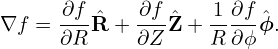 | (12) |
Since ∇f is axisymmetric, it follows that all the three components of ∇f are independent of ϕ, i.e., ∂2f∕∂R∂ϕ = 0, ∂2f∕∂Z∂ϕ = 0, and ∂2f∕∂ϕ2 = 0, which implies that ∂f∕∂ϕ is independent of R, Z, and ϕ, i.e., ∂f∕∂ϕ is actually a spatial constant. Using this, the ϕ component of the gauge transformation (11) is written
where C is a constant. Note that the requirement of being axial symmetry greatly reduces the degree of freedom of the gauge transformation for Aϕ (and thus for RAϕ, i..e, Ψ). Multiplying Eq. (13) with R, we obtain the corresponding gauge transformation for Ψ,
 | (14) |
which indicates Ψ has the same gauge transformation as the electric potential, i.e., adding a constant. (Note that the definition Ψ(R,Z) ≡ RAϕ does not imply Ψ(R = 0,Z) = 0 because Aϕ can adopt 1∕R dependence under the gauge transformation (13)).
