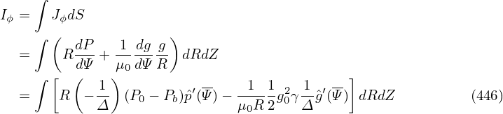
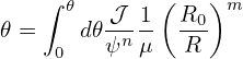
Grad-Shafranov equation with prescribed safety factor proﬁle (to be ﬁnished)

15.10 Grad-Shafranov equation with prescribed safety factor proﬁle (to be ﬁnished)

In the GS equation, g(Ψ) is one of the two free functions which can be prescribed by users. In some cases, we want to specify the safety factor proﬁle q(Ψ), instead of g(Ψ), in solving the GS equation. Next, we derive the form of the GS equation that contains q(Ψ), rather than g(Ψ), as a free function. The safety factor deﬁned in Eq. (160) can be written

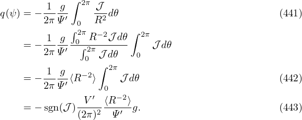
1 g ∫ 2π𝒥 q(ψ) = − 2πΨ-′ R2-d𝜃 (441) ∫02π −2 ∫ 2π = − 1--g -0∫R---𝒥d𝜃- 𝒥d𝜃 2πΨ ′ 02π𝒥 d𝜃 0 ∫ 2π = − 1--g′⟨R −2⟩ 𝒥d𝜃 (442) 2πΨ 0 = − sgn(𝒥 )-V-′-⟨R−2⟩g. (443) (2π)2 Ψ ′

Equation (443) gives the relation between the safety factor q and the toroidal ﬁeld function g. This relation can be used in the GS equation to eliminate g in favor of q, which gives

(2π)2 g = − sgn(𝒥 )-′-−2-Ψ ′q. V ⟨R ⟩

(444)

[ ] -dg -(2π)2-- --(2π-)2-- ′ ⇒ dΨ g = V′⟨R −2⟩q V ′⟨R −2⟩qΨ ψ.

(445)

Note that this expression involves the ﬂux surface average, which depends on the ﬂux surface shape and the shape is unknown before Ψ is determined.

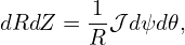
Multiplying Eq. (573) by R⁻² gives

[ ] 1 ( 𝒥 ) ( 𝒥 ) dp dg 𝒥- Ψ′R2|∇ψ |2 + Ψ ′R2(∇ψ ⋅∇ 𝜃) + μ0dΨ-+ R −2dΨ-g = 0. ψ 𝜃

(446)

Surface-averaging the above equation, we obtain

[ ] 2π∫ ( ′ 𝒥 2) ( ′ 𝒥 ) dp −2 dg V′- d𝜃 Ψ R2-|∇ψ| + Ψ R2-(∇ψ ⋅∇𝜃) + μ0dΨ-+ ⟨R ⟩dΨ-g = 0, ψ 𝜃

(447)

∫ ( ) ⇒ 2π-- d𝜃 Ψ′-𝒥-|∇ ψ|2 +μ0 dp-+ ⟨R −2⟩dgg = 0, V′ R2 ψ dΨ dΨ

(448)

[ ( ) ] 2π- ′∫ |∇ψ-|2 -dp −2 dg- ⇒ V′ Ψ d𝜃 𝒥 R2 ψ + μ0dΨ + ⟨R ⟩dΨg = 0,

(449)

[ ⟨ ⟩ ] 1-- ′ ′ |∇ψ-|2 -dp −2 dg- ⇒ V′ V Ψ R2 ψ + μ0dΨ + ⟨R ⟩dΨg = 0.

(450)

[ ⟨ 2⟩] ⇒ V′Ψ′ |∇-ψ2|- + μ0V′ dp-+ ⟨R−2⟩V′ dg-g = 0, R ψ dΨ dΨ

(451)

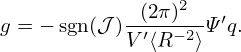
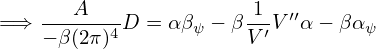
Substitute Eq. (445) into the above equation to eliminate gdg∕dΨ, we obtain

[ ⟨ ⟩ ] [ ] ′ ′ |∇ψ|2 ′dp- 4 --qΨ-′-- ⇒ V Ψ R2 ψ + μ0V dΨ + q(2π) V ′⟨R− 2⟩ ψ = 0,

(452)

Eq. (452) agrees with Eq. (5.55) in Ref. [16].

⟨ ⟩ [ ⟨ ⟩] [ ] [ ] ⇒ V ′ |∇ψ-|2 Ψ′′+ V′ |∇-ψ|2 Ψ′+μ V ′ dp+q (2π)4 ---q----Ψ ′′+q (2π)4 ---q---- Ψ′ = 0 R2 R2 ψ 0 dΨ V′⟨R −2⟩ V′⟨R−2⟩ ψ

(453)

{ } ′′ 1 [ ′⟨|∇ψ |2⟩ ] ′ 4[ q ] ′ ′ dp ⇒ Ψ = −V-′D V --R2- Ψ +q(2π) V-′⟨R-−2⟩ Ψ + μ0V dΨ- ψ ψ

(454)

where

⟨|∇ ψ|2⟩ (2π )4 ( q )2 D = ---2- + ---−2 --′ R ⟨R ⟩ V

(455)

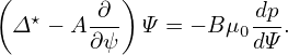
The GS equation is

△ ⋆Ψ = − μ R2 dp-− g dg 0 dΨ dΨ

(456)

4 [ ′ ] ⇒ △ ⋆Ψ = − μ0R2-dp− q(2π)-----qΨ---- dΨ V′⟨R −2⟩ V ′⟨R −2⟩ ψ

(457)

4 { [ ] [ ] } ⇒ △ ⋆Ψ = − μ0R2-dp− q(2π)--- ---q---- Ψ′ + ---q---- Ψ′′ dΨ V′⟨R −2⟩ V ′⟨R−2⟩ ψ V ′⟨R− 2⟩

(458)

Using Eq. (454) to eliminate Ψ′′ in the above equation, the coeﬃcients before (−μ₀dp∕dΨ) is written as

{ [ ] } B = R2 − -q(2π)4-- ---q---- -1--V′ V′⟨R −2⟩ V′⟨R−2⟩ V′D 1 { 2 ( q )2 (2π)4 } = D- R D − V-′ ⟨R−-2⟩2 . (459)

Substituting the expression of D into the above equation, we obtain

{ ⟨ ⟩ ( ) ( ) } B = -1 R2 |∇ψ-|2 + R2 (2π)4- q--2 − q--2-(2π)4 D R2 ⟨R −2⟩ V′ V′ ⟨R −2⟩2 1 { 2 ⟨|∇ψ |2⟩ ( q )2 (2π)4 ( 2 1 ) } = D- R --R2- + V-′ ⟨R−-2⟩ R − ⟨R−2⟩ , (460)

which is equal to the expression (5.58) in Ref. [16]. The coeﬃcient before Ψ′ is written as

A = −

{[ ] [ ] [( ⟨ 2⟩ ) [ ] ]}
-′-q−2-- − -′-q−2----1′- V ′ |∇ψ2| + q(2π)4 -′-q−2--
V ⟨R ⟩ ψ V ⟨R ⟩ V D R ψ V ⟨R ⟩ ψ

Deﬁne

α =

β =

A = −(2π)⁴β

D 1 ′ 4 =⇒ −-(2π)4β-A = Dβψ − βV-′[(V α)ψ +q(2π) βψ]

(461)

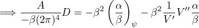
= ⇒ ---D----A = D β − β-1[V′′α + V ′α + q(2π )4β ] − β(2π)4 ψ V ′ ψ ψ

(462)

Using

D = α + (2π )4⟨R− 2⟩β2

(463)

Eq. () is written as

] =⇒ ---D---A = αβ + (2π)4⟨R −2⟩β2β − β-1-V′′α − β-1V ′α − β 1-q(2π )4β − β(2π)4 ψ ψ V ′ V ′ ψ V′ ψ

(464)

D 4 −2 2 1 ′′ 1 4 ] =⇒ −-β(2π-)4A = α βψ + (2π) ⟨R ⟩β βψ − β V′V α − βαψ − βV-′q(2π) βψ

(465)

A 1 −-β(2π)4D = αβψ + (2π )4⟨R− 2⟩β2βψ − βV-′V ′′α − β αψ − β2⟨R −2⟩(2π)4βψ

(466)

A 1 ′′ = ⇒ −-β(2π)4-D = αβψ − βV′V α− βα ψ

(467)

( ) =⇒ ---A---D = − β2 α- − β 1-V ′′α − β(2π)4 β ψ V′

(468)

A (α ) 1 α =⇒ − β(2π)4D = − β2 β − β2V-′V ′′β- ψ

(469)

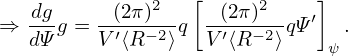
[ ] A (α ) 1 α =⇒ −-β(2π)4D = − β2 -β + V-′V ′′β- ψ

(470)

[( ) ] ---A---- 2-1- α- ′ ′′α- = ⇒ − β(2π)4 D = − β V ′ β ψV + V β

(471)

A 1 (α ) =⇒ − β(2π)4D = − β2V-′ β-V′ ψ

(472)

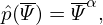
4 ( )3 [⟨ 2⟩ −2 ] =⇒ A = (2π)- ----q--- 1-- |∇-ψ|- ⟨R--⟩V ′2 D V ′⟨R −2⟩ V′ R2 q ψ

(473)

But the expression of A is slightly diﬀerent from that given in Ref. [16] [Eq. (5.57)]. Using the above coeﬃcients, the GS equation with the q-proﬁle held ﬁxed is written as

( ) Δ⋆ − A-∂- Ψ = − B μ0 dp. ∂ψ dΨ

(474)

[prev] [prev-tail] [front] [up]