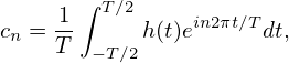
In the above, we go through the process “Fourier series→Fourier transformation →DFT”, which corresponds to going from the discrete case (Fourier series) to the continuous case (Fourier transformation), and then back to the discrete case (DFT). Since both Fourier series and DFT are discrete in frequency, it is instructive to examine the relation between the Fourier coefficient cn and the DFT Hn. The Fourier coefficient of h(t) is given by Eq. (93), i.e.,
|
| (77) |
which can be equivalently written
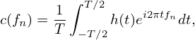 | (78) |
where fn = n∕T. On the other hand, if h(t) is sampled with sampling rate fs = 1∕Δ, then the number of sampling points per period is N = T∕Δ. Then the frequency at which the Fourier transform H(f) is evaluated in getting the DFT [Eq. (36)] is written
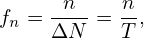 | (79) |
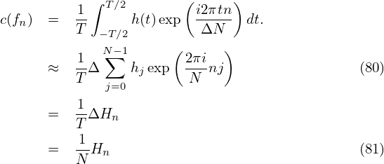
which is identical to the frequency to which the Fourier coefficient cn corresponds. Using fn = n∕(ΔN) in Eq. (78), we obtain
i.e., dividing the DFT Hn by N gives the corresponding Fourier expansion coefficient cn. We can further use Eqs. (29) and (30) to recover the Fourier coefficients in terms of trigonometric functions cosine and sine,Note that the approximation in Eq. (80) becomes an exact relation if the largest frequency contained in h(t) is less than 1∕(2Δ).