C.4 Computing Fourier integrals using FFT (not finished, to be deleted)

Consider the calculation of the following integral:

      ∫ b
I(ω ) =   eiωth(t)dt.
       a
(138)

Divide the interval [a,b] into M uniform sub-intervals and define

    b− a
Δ = ----,tj = a + Δj,hj = h(tj),j = 0,1,2,...,M
     M
(139)

Then the integration in Eq. (138) can be approximated as

         M−1
I(ω) ≈ Δ ∑  hj exp (iωtj).
         j=0
(140)

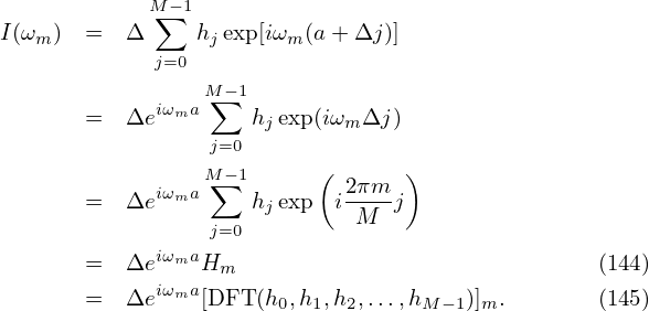
Define ωm = 2πm∕(MΔ) with integer m and M∕2 < m < M∕2. Consider the calculation of I(ωm). Using Eq. (140), we obtain

            M∑ −1
I(ωm)  =  Δ     hjexp[iωm (a+ Δj)]
             j=0
             iω a M∑−1
       =  Δe  m      hjexp(iωm Δj)
                 j=0
             iω a M∑−1      ( 2πm  )
       =  Δe  m      hjexp i-M--j
                 j=0
       =  ΔeiωmaHm                               (141)
       =  Δeiωma[DFT (h0,h1,h2,...,hM −1)]m.        (142)
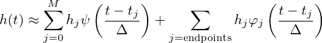
Equation (142) indicates the value of the integration I(ωm) can be obtained by calculating the discrete Fourier transformation of hj. However, as discussed in Ref. [2], equation (142) is not recommended for practical use because the oscillatory nature of the integral will make Eq. (142) become systematically inaccurate as ω increases. Next, consider a new method, in which h(t) is expanded as
      M     (      )               (      )
h(t) ≈ ∑ hjψ  t−-tj  +   ∑     hjφj  t−-tj
      j=0       Δ      j=endpoints        Δ
(143)

Apply the integral operator abdtexp(iωt) to both sides of Eq. (143), we obtain

∫ b    iωt    ∑M    ∫ b ( t− tj) iωt     ∑       ∫ b   (t − tj) iωt
   h(t)e  dt ≈   hj    ψ  -Δ--- e  dt+         hj   φj  --Δ--  e  dt.
 a           j=0    a                 j=endpoints    a
(144)

Make the change of variables s = (ttj)Δ in the first integral and s = (ta)Δ in the second integral, the above equation is written as

∫ b            ∑M    ∫ b                   ∑       ∫ b
   h(t)eiωtdt ≈ Δ   hj    ψ(s)eiω(Δs+tj)ds+ Δ         hj   φj (s− j)eiω(Δs+a)ds
 a             j=0    a                  j=endpoints    a
(145)

Define 𝜃 = ωΔ and make use of tj = a + jΔ, the above equation is written as

∫ b    iωt       iωa M∑    i𝜃j∫ b    i𝜃s     iωa   ∑       ∫ b        i𝜃s
 a h(t)e  dt ≈ Δe      hje   a ψ(s)e  ds+ Δe            hj a φj(s− j)e ds
                   j=0                        j=endpoints
(146)

Define

       ∫ b
W (𝜃) =   ψ (s)ei𝜃sds
        a
(147)

       ∫ b
αj(𝜃) =   φj(s− j)ei𝜃sds
        a
(148)

Then Eq. (146) is written as

                   ⌊                               ⌋
∫ b     iωt       iωa⌈     ∑M    i𝜃j    ∑            ⌉
  a h (t)e dt ≈ Δe    W (𝜃)   hje   +         hjαj(𝜃) .
                         j=0        j=endpoints
(149)


pict

Figure 9: Older version of Fig. 2, created by Metapost, the new version is created by the vector graphic editor in TeXmacs.