![δB ⊥ = ∇ × δA − (e∥ ⋅∇ × δA)e∥
= ∇ × (δA + δA e )− [e ⋅∇ × (δA + δA e )]e (306)
⊥ ∥ ∥ ∥ ⊥ ∥ ∥ ∥](nonlinear_gyrokinetic_equation365x.png)
Note that
![( ∂δA ) (∂δA ) 1 [ ∂ ∂δA ]
∇ × δA ⊥ = − ---ϕ- er + ----r eϕ +- --(rδAϕ)− ----r e∥.
∂z ∂z r ∂r ∂ ϕ](nonlinear_gyrokinetic_equation367x.png) | (309) |
Note that the parallel gradient operator ∇∥≡ e∥⋅∇ = ∂∕∂z acting on the the perturbed quantities will result in quantities of order O(λ2). Retaining terms of order up to O(λ), equation (309) is written as
![1 [ ∂ ∂ δA ]
∇ ×δA ⊥ ≈ - --(rδAϕ)− ----r e∥,
r ∂r ∂ ϕ](nonlinear_gyrokinetic_equation368x.png) | (310) |
i.e., only the parallel component survive, which exactly cancels the last term in Eq. (308), i.e., equation (308) is reduced to
 | (311) |
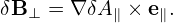
In terms of δBxL and δByL, δB⊥ is written as
 | (312) |
Dotting the above equation by ∇x and ∇y, respectively, we obtain
 | (313) |
 | (314) |
Equations (313) and (314) can be further written as
 | (315) |
and
 | (316) |
The solution of this 2 × 2 system is expressed by Cramer’s rule in the code.
Use B0 = Ψ′∇x ×∇y
b = Ψ′∇x ×∇y∕B0

![( ) ( ) [ ]
∂δA-ϕ ∂δAr- 1 ∂-- ∂δAr-
∇ × δA⊥ = − ∂z er + ∂z er + r ∂r(rδAϕ)− ∂ϕ e∥](nonlinear_gyrokinetic_equation377x.png) | (319) |
Note that the parallel gradient operator ∇∥≡ e∥⋅∇ = ∂∕∂z acting on the the perturbed quantities will result in quantities of order O(λ2). Retaining terms of order up to O(λ), equation (309) is written as
![1 [ ∂ ∂ δA ]
∇ ×δA ⊥ ≈ - --(rδAϕ)− ----r e∥,
r ∂r ∂ ϕ](nonlinear_gyrokinetic_equation378x.png) | (320) |
Using this, equation (318) is written as
![1[ ∂ ∂δA ]
δB∥ = - --(rδA ϕ)− ----r .
r ∂r ∂ϕ](nonlinear_gyrokinetic_equation379x.png) | (321) |
However, this expression is not useful for GEM because GEM does not use the local coordinates (r,ϕ,z).]
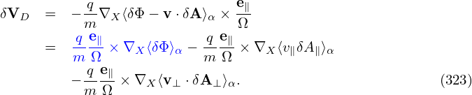
The perturbed drift δVD is given by Eq. (138), i.e.,
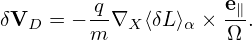 | (322) |
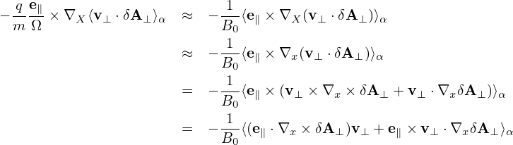
Using δL = δΦ − v ⋅ δA, the above expression can be further written as
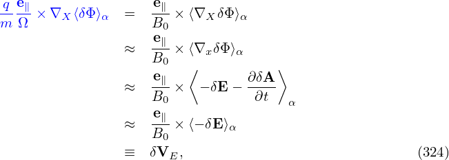
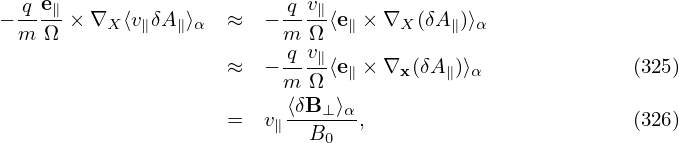
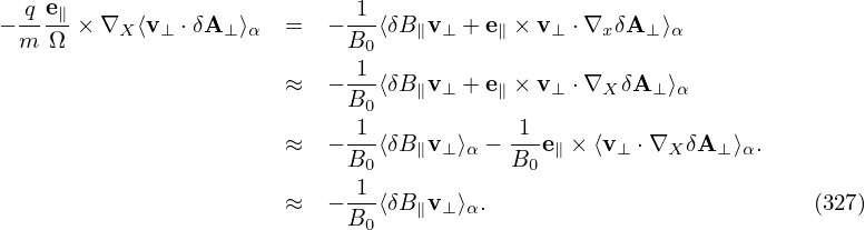
Accurate to order O(λ), the term involving δΦ is which is the δE×B0 drift. Accurate to O(λ), the ⟨v∥δA∥⟩α term on the right-hand side of Eq. (323) is written which is called “magnetic fluttering” (this is actually not a real drift). In obtaining the last equality, use has been made of Eq. (311), i.e., δB⊥ = ∇xδA∥× e∥.Accurate to O(λ), the last term on the right-hand side of expression (323) is written
Using Eqs. (324), (326), and (327), expression (323) is finally written as
 | (328) |
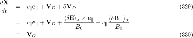
Using this, the first equation of the characteristics, equation (292), is written as
[Note that
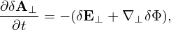 | (331) |
where ∂δA⊥∕∂t is of O(λ2). This means that δE⊥ + ∇⊥δϕ is of O(λ2) although both δE⊥ and δϕ are of O(λ).]
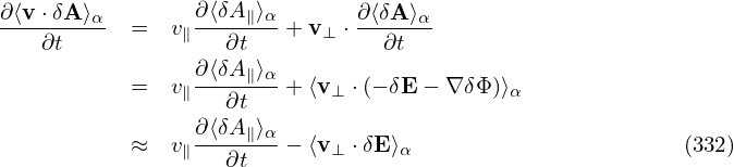
Note that
where use has been made of ⟨v⊥⋅∇δϕ⟩≈ 0, This indicates that ⟨v⊥⋅ δE⟩α is of O(λ1)δE. Using Eq. (332), the coefficient before ∂F0∕∂𝜀 in Eq. (141) can be further written as Using Eq. (333) and (), gyrokinetic equation (141) is finally written as![δB ≈ ∇ × δA +∇ δA × e − [e ⋅∇ × δA + e ⋅(∇δA × e )]e (307)
⊥ ⊥ ∥ ∥ ∥ ⊥ ∥ ∥ ∥ ∥
= ∇ × δA ⊥ +∇ δA∥ × e∥ − (e∥ ⋅∇ × δA⊥ )e∥ (308)](nonlinear_gyrokinetic_equation366x.png)

![[ ( ) ]
−-q − ∂⟨v-⋅δA⟩α − v e + V − -qe∥ × ∇ ⟨v⋅δA ⟩ ⋅∇ ⟨δΦ⟩
m ∂t ∥ ∥ D m Ω X α X α
q [ ∂⟨δA∥⟩α ( qe∥ ) ⟨ ∂δA ⟩ ]
= −m- − v∥--∂t-- + ⟨v⊥ ⋅δE⟩α − v∥e∥ + VD − m-Ω × ∇X ⟨v⋅δA ⟩α ⋅ − δE −-∂t-
[ ( ) ⟨ α ⟩ ]
≈ −-q − v∥∂⟨δA∥⟩α + ⟨v⊥ ⋅δE⟩α − v∥e∥ + VD −-qe∥ × ∇X ⟨v⋅δA ⟩α ⋅⟨− δE ⟩α + v∥ ∂A∥-
m [ ∂t ( m Ω ) ] ∂t α
= −-q ⟨v⊥ ⋅δE⟩α + v∥e∥ + VD − -qe∥ × ∇X ⟨v⋅δA ⟩α ⋅⟨δE⟩α
m [ ( m Ω ) ]
≈ −-q ⟨v ⋅δE⟩ + v e + V + v ⟨δB-⊥⟩ ⋅⟨δE ⟩ . (333)
m ⊥ α ∥ ∥ D ∥ B0 α](nonlinear_gyrokinetic_equation390x.png)
![[ ( ) ]
-∂ + v∥e∥ + VD + ⟨δE-⟩α ×-e∥-+ v∥ ⟨δB-⊥⟩α ⋅∇X δf
∂t B0 B0
( ⟨δE-⟩α ×-e∥ ⟨δB-⊥⟩α)
= − B0 + v∥ B0 ⋅∇XF0
q [ ( ⟨δB ⟩ ) ] ∂F
− -- ⟨v⊥ ⋅δE⟩α + v∥e∥ + VD + v∥---⊥-α- ⋅⟨δE⟩α --0. (334)
m B0 ∂ 𝜀](nonlinear_gyrokinetic_equation391x.png)