F Implementation of gyrokinetics in particle-in-cell (PIC) codes

F.1 Monte-Carlo evaluation of distribution function moment at grid-points

Suppose that the 6D guiding-center phase-space (X,v) is described by (ψ,𝜃,ϕ,v_∥,α,v_⊥) coordinates, where α is the gyro-angle. Denote the Jacobian of the coordinate system by 𝒥_rv.

Suppose that we sample the 6D phase-space by using a probability function P(ψ,𝜃,ϕ,v_⊥,α,v_∥). (Then the effecitive probability function used in rejection method is P𝒥_r𝒥_v.) Note that we will sample a distribution function δf_g(X,v_⊥,v_∥,α) that happens to be independent of the gyro-angle α. Since δf_g is uniform in α, it is natural to smaple α using a uniform probability function, i.e., P(X,v_⊥,α,v_∥) can be chosen to be independent of α. Then the weight is also independent of α. In terms of sampling δf_g, there is no need to specify α because both f_g and marker distribution g = N_pP are indepedent of α. However, sampling α is still necessary in simulations. From the perspective of programming, it is ready to understand why α needs to be specified: when computing density at grid-points, we need to compute particle locations from the guiding-center locations which requires us to specify the gyro-angle α for each marker. Specifically, markers in guiding-center space (X,v_⊥,α,v_∥) with fixed (X,v_⊥,v_∥) but different values of α correspond to markers in particle space with different locations (and different α′). In the PIC method of computing δn or δj_∥ at fixed x, the contribution of each particle marker to the density is affected by the distance of the particle marker to the fixed x. Therefore different values of α contributes differently to δn or δj_∥, and thus the resolution of α matters.

For a marker with coordinators (X,v_⊥,v_∥,α), the corresponding particle position can be calculated by using the inverse guiding-center transformation (29). Then we can deposit the marker weight to grid-points in the same way that we do in conventional PIC simulations. Looping over all markers, we build the particle density at grids.

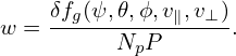
Compared with conventional PIC methods, where particle positions are directly sampled, what is the benefit of sampling guiding-center positions and then transform them back to the particle positions? More computations are involved since we need to numerically perform the inverse guiding-center transformation. The answer lies in the important fact that the distribution function f_g(X,v_⊥,v_∥,α) that needs to be numerically evaluated in gyrokinetic simulation is actually independent of the gyro-angle α. Furthermore, we use a probability density function P that is independent of α to sample the 6D phase space (X,v_⊥,v_∥,α). Then the marker weight w ≡ f_g∕(N_pP) is independent of α, where N_p is number of markers loaded. This fact enable resolution in particle coordinates can be increased in a trivial way, as described below.

Suppose we have a concrete sampling of f_g in the 6D phase-space (X,v_⊥,v_∥,α), i.e., (X_j,v_⊥j,v_∥j,α_j,w_j) with j = 1,…,N_p, then we can do the inverse guiding-center transform and then deposit particles to the grids to obtain a moment (e.g. density).

Since P𝒥_rv is independent of α, the sampling α_j with j = 0,1,…,N_p are uniform distributed random numbers. Therefore we can generate another sampling of α (denoted by α_j′ with j = 1,…,N_p) using random number generators and combine α_j′ with the old sampling (X_j,v_⊥j,v_∥j) to obtain a new sampling (X_j,v_⊥j,v_∥j,α_j′,w_j′).  The values of w at the new sampling points are equal to the original values, i.e., w_j′ = w_j since the particle weight w = f_g∕(N_pP) is independent of α.  Using the new sampling and following the same procedures given above, we can estimate values of the moment at grid-points again, which will differ from the estimation obtained using the old sampling because the resulting sampling of x and α′ for f_p is different. Taking the average of the two estimations will give a more accurate estimation because the resolution in x and α′ for f_p is increased.

[Note that even if P𝒥_rv is dependent on α due to the possible dependence of 𝒥_rv on α, we still can easily generate a new set of sampling which differs from the old sampling only in α. Specifically, in the rejection method, we use the old sampling (X_j,v_⊥j,v_∥j) for each reject step and only adjust α to satisfy the acceptance criteria.]

We can also construct a new sampling by replacing α_j with α_j + Δ, where Δ is a constant. Then the new set of sampling (X_j,v_⊥j,v_∥j,α_j + Δ,w_j) with j = 1,…,N_p is still a consistent set of sampling.

In doing the deposition, each marker has a single gyro-angle. Due to the independence of the weight (w = f_g∕(N_pP)) of the gyro-angle, the particle phase space resolution can be increased in a way that there can be several gyro-angles for a single (X_j,v_⊥j,v_∥j). This gives the wrong impression that the gyro-angle of a guiding-center marker is arbitrary. The correct understanding is that given above, i.e., we do several (say 4) separate sampling of the phase space and then average the results.

In the code, the gyro-angle is defined relative to the direction ∇ψ∕|∇ψ| at the guiding-center position. Specifically, the gyro-angle is defined as the included angle between ∇ψ∕|∇ψ| and −v × e_∥(x)∕Ω(x), where e_∥(x)∕Ω(x) is approximated by the value at the guiding-center location.

Then (X_j,v_⊥j,v_∥j) can be evolved by using the guiding-center motion equation. (It is obvious how to evalute the gyro-averaging of the electromagnetic fields needed in pusing markers.)

F.2 Monte-Carlo sampling of 6D guiding-center phase-space

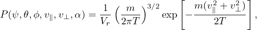
Suppose that the 6D guiding-center phase-space (X,v) is described by (ψ,𝜃,ϕ,v_∥,v_⊥,α) coordinates. The Jacobian of the coordinate system is given by 𝒥 = 𝒥_rv_⊥, where 𝒥_r = 𝒥 (ψ,𝜃) is the Jacobian of the coordinates (ψ,𝜃,ϕ). Suppose that we sample the 6D phase-space by using the following probability density function:

(345)

where V _r is the volume of the spatial simulation box, T is a constant temperature. P given above is independent of ψ,𝜃,ϕ and α. It is ready to verify that the above P satisfies the following normalization condition:

(346)

I use the rejection method to numerically generate N_p markers that satisfy the above probability density function. [The effective probability density function actually used in the rejection method is P′, which is related to P by

(347)

Note that P′ does not depend on the gyro-angle α.]

Then the weight of a marker sampling δf_g is written as

(348)

Since both f_g and P are independent of the gyro-angle α, w is also independent of α.

The numerical representation of δf_g is written

(349)

Although the distribution function δf_g to be sampled is independent of the gyro-angle α, we still need to specify the gyro-angle because we need to use the inverse guiding-center transformation, which needs the gyro-angle. Each marker needs to have a specific gyro-angle value α_j so that we know how to transform its X_j to x_j and then do the charge deposition in x space.

To increase the resolution over the gyro-angle (the quantity of intest to us, e.g., density, is the integration of the particle distribution function at fixed spatial location, and the distribution at the fixed location is not uniform in the gyro-angle. So the resolution over α matters), we need to load more markers. However, thanks to the fact that both sampling probability density function P and δf_g are independent of α, the resolution over the gyro-angle can be increased in a simple way.

(350)

This corresponds to sampling the 6D phase-space 4 separate times (each time with identical sampling points in (X,v_∥,v_⊥) but different sampling points in α) and then using the averaging of the 4 Monte-Carlo integrals to estimate the exact value. This estimation can also be (roughly) considered as a Monte-Carlo estimation using 4 times larger number of markers as that is originally used (the Monte-Carlo estimation using truly 4 time larger number of markers is more accurate than the result we obtained above because the former also increase the resolution of (X,v_∥,v_⊥) while the latter keeps the resolution of (X,v_∥,v_⊥) unchanged.)

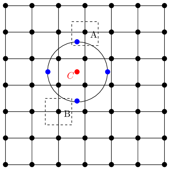
In numerical implementation, we choose N sampling points that are evenly distributed on the gyro-ring (N is usually 4 as a compromise between efficiency and accuracy). And the weight is evenly split by the N sub-markers on the gyro-ring. Therefore each sub-marker have a Monte-Carlo weight w_j∕N, where w_j is the weight of the j th marker. Then calculating the integration (356) at a grid corresponds to depositing all the N sub-markers associated with each guiding-center marker to the grid, as is illustrated in Fig. 6. However, interpreting in this way is confusing to me because: why can you split a single sampling into N different samplings? I prefer the above interpretation that the 6D phase space is sampled 4 separate times and thus we get 4 estimations and finally we take the averaging of these 4 estimations. It took a long time for me to finally find this way of understanding.

In summary, the phase-space to be sampled in gyrokinetic simulations are still 6D rather than 5D. In this sense, the statement that gyrokinetic simulation works in a 5D phase space is misleading. We are still working in the 6D phase-space. The only subtle thing is that the sixth dimension, i.e., gyro-angle, can be sampled in an easy way that is independent of the other 5 variables.

In numerical implementation, the gyro-angle may not be explicitly used. We just try to find 4 arbitrary points on the gyro-ring that are easy to calculate. Some codes (e.g. ORB5) introduces a random variable to rotate these 4 points for different markers so that the gyro-angle can be sampled less biased.

From the view of particle simulations, the gyrokinetic model can be considered as a noise reduction method, where the averaging over the gyro-angle is equivalent to a time averaging over a gyro-period, which reduces the fluctuation level (in both time and space) associated with evaluating the Monte-Carlo phase integration. Here the averaging in gyrokinetic particle simulation refers to taking several points on a gyro-ring when depositing markers to spatial grids to obtain the density and current on the grids. (Another gyro-averaging appears in evaluating the guiding-center drift.) In gyrokinetic particle simulation, even a step size smaller than a gyro-period is taken, the quantities used in the model is still the ones averaged over one gyro-period. In this sense, a gyrokinetic simulation is only meaningful when the time step size is larger than one gyro-period. [**Some authors may disagree with that the gyro-averaging is a time-averaging. They may consider the gyro-averaging as the phase-space integration over the gyro-angle coordinate. This view seems to be right in Euler simulations but seems to be wrong in particle simulations. The reason is as follows. For each marker, choose a random gyro-phase and then do the inverse transformation to obtain particle position, and sum over all markers (this corresponds to phase-space Monte-Carlo integration, which include the gyro-angle integration, so no further gyro-angle integration is needed); choose another random gyro-phase and repeat the above procedure (this can be interpreted as do the phase-space Monte-Carlo integration at another time), choose further random gyro-phase for each marker and repeat. Finally averaging all the above values to obtain the final estimation of the phase-space integration. This amounts to a time-averaging over a gyro-motion. In summary, sampling several times with different gyro-phases for each marker and taking the average amounts to the time averaging over gyro-motion**]

When doing the time-average over the ion cyclotron motion, the time variation of the low-frequency mode is negligible and only the spatial variation of the modes is important. For the gyro-motion, only the gyro-angle is changing and all the other variables, (X,v_⊥,v_∥),  are approximately constant. As a result, this time averaging finally reduces to a gyro-averaging.

I prefer to reason in terms of particle position and velocity, and consider the guiding-center location as an image of the particle position. When working in the guiding-center coordinates, I prefer to reason by transforming back to the particle position. This reasoning is clear and help me avoid some confusions I used to have.

F.3 Distribution function transform**check

In the above, we assume that X and x are related to each other by the guiding-center transformation (27) or (29) , i.e., x and X are not independent. For some cases, it may be convenient to treat x and X as independent variables and express the guiding-center transformation via an integral of the Dirac delta function. For example,

(351)

where x and X are considered as independent variables, ρ is the gyroradius evaluated at x, δ³(x − X − ρ) is the three-dimensional Dirac delta function. [In terms of general coordinates (x₁,x₂,x₃), the three-dimensional Dirac delta function is defined via the 1D Dirac delta function as follows:

(352)

where 𝒥 is the the Jacobian of the general coordinate system. The Jacobian is included in order to make δ³(x) satisfy the normalization condition ∫ δ³(x)dx = ∫ δ³(x)|𝒥|dx₁dx₂dx₃ = 1.]

Expression (351) can be considered as a transformation that transforms an arbitrary function from the guiding-center coordinates to the particle coordinates. Similarly,

(353)

is a transformation that transforms an arbitrary function from the the particle coordinates to the guiding-center coordinates.

F.4 Moments of distribution function expressed as integration over guiding-center variables

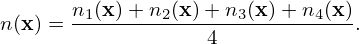
In terms of particle variables (x,v), it is straightforward to calculate the moment of the distribution function. For example, the number density n(x) is given by

(354)

However, it is a little difficult to calculate n(x) at real space location x by using the guiding-center variables (X,v). This is because holding x constant and changing v, which is required by the integration in Eq. (354), means the guiding-center variable X is changing according to Eq. (27). Using Eq. (34), expression (354) is written as

(355)

As is mentioned above, the dv integration in Eq. (355) should be performed by holding x constant and changing v, which means the guiding-center variable X = X(x,v) is changing. This means that, in (X,v) space, the above integration is a (generalized) curve integral along the the curve  X(v) = x −ρ(x,v) with x being constant. Treating X and x as independent variables and using the Dirac delta function δ, this curve integral can be written as the following double integration over the independent variables X and v:

(356)

Another perspective of interpreting Eq. (356) is that we are first using the transformation (351) to transform f_g to f_p and then integrating f_p in the velocity space.