Write the distribution function F as
|
| (84) |
where F0 is the equilibrium distribution function. Then Eq. (78) is written as
 | (85) |
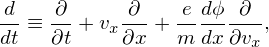
Use the definition of the orbit propagator,
 | (86) |
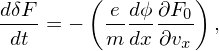
to rewrite the right-hand side of Eq. (85), yielding
 | (87) |
which can be integrated to obtain the time evolution of δF.
The time evolution of δF can also be obtained by using
 | (88) |
In this way, the time integration of δF∕dt is avoided, which may reduce the computational work load and improve the accuracy of δF. This seemingly trivial method was emphasized in a CPC paper[1], which introduces an adaptive F0 method based on this idea. I have compared the results of Landau damping obtained by the two methods (i.e., using Eq. (87) and Eq. (88), respectively), which shows they agree with each other very well.