The effective field on a marker is defined as the averaged field on the group of particles represented by the marker. To get the averaged field, we need to reconstruct a continuum electric field from the field values on the discrete grids.
One of many methods of reconstructing the continuum electric field is to assume that the field is constant in each cell, i.e., piecewise constant function, i.e.,
|
| (45) |
where Ei,j,k is the field value at grid-points (centers of cells) obtained by solving the field equation. The electric field on a computational marker is the average of the electric field over all the physical particles contained in the marker, i.e.,
 | (46) |
Using fp given in Eq. (22) in the above equation, we obtain
![∫ ∫ ∫ [ ( ) ][ ( )] [ ( ) ]
+∞ +∞ +∞ -1-- α-−-αp -1-- β-−-βp -1-- γ −-γp
Ep = − ∞ − ∞ − ∞ E (α,β,γ) Δ αpS1D Δ αp Δ βpS1D Δ βp ΔγpS1D Δγp dαdβdγ,](particle_simulation47x.png) | (47) |
where the Jacobian and wp disappear. Use the reconstructed electric field [Eq. (45)] in the above equation, giving
 | (48) |
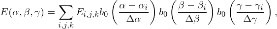
If we choose the shape function S1D as the b-spline function bl with Δαp = Δα, Δβp = Δβ, and Δγp = Δγ, then the above equation is written as
 | (49) |
which specifies how the effective field on a marker is related to the nearby field on the grid-points.
Another way of reconstructing the continuum electric field is to assume that the field is linear function between grids. In this case, if the spatial shape function of markers is Dirac delta function, then it is obvious that the effective field on a marker can be obtained by linearly interpolating the fields on the nearyby grids. If the spatial shape function of markers is b0, what is the interpolation scheme of obtaining the effective field on a marker? To be worked out. The result will be a little complicated than the linear interpolation and thus involves more computational overhead. The benefit can be that the noise can be further reduced, compared with the linear interpolation.