Next: Periodic conditions of physical Up: Field-line-following coordinates Previous: Definition of the field-line-following
I am now developing a fully kinetic ions module in electromagnetic turbulence
code GEM which uses field-line-following coordinates. Having an accurate
understanding of the field-line-following coordinates is importan for writing
the code. In this section, I try to visualize some aspects of the coordinates
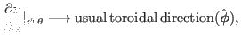
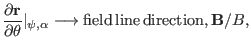
which are helpful for writing correct codes. The directions of the covariant
basis vectors of
![]() coordinates are as follows:
coordinates are as follows:
|
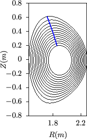
The relation
![]() given by Eq.
(284) indicates that the toroidal shift for a radial change form
given by Eq.
(284) indicates that the toroidal shift for a radial change form
![]() to
to ![]() is given by
is given by
![]() , which is
larger on
, which is
larger on ![]() isosurface with larger value of
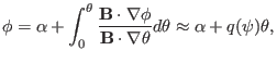
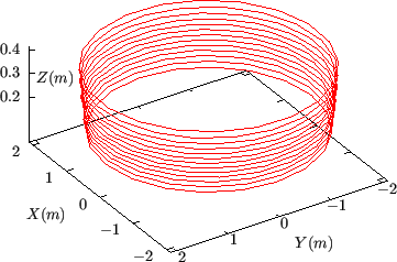
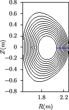
isosurface with larger value of ![]() . An example for
this is shown in Fig. 16, which has larger toroidal shift than
that in Fig. 15.
. An example for
this is shown in Fig. 16, which has larger toroidal shift than
that in Fig. 15.
|
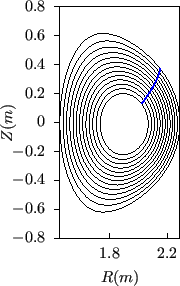
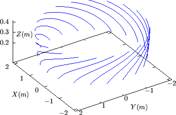
The
![]() lines
can be understood in another way. Examine a family of magnetic field lines
that start from the low-field-side midplane (
lines
can be understood in another way. Examine a family of magnetic field lines
that start from the low-field-side midplane (
![]() ) with the same
toroidal angle
) with the same
toroidal angle
![]() but different radial coordinates. When these
field lines travel to an isosurfce of
but different radial coordinates. When these
field lines travel to an isosurfce of ![]() with
with
![]() , the
intersecting points of these field lines with the
, the
intersecting points of these field lines with the ![]() isosurface will
trace out a
isosurface will
trace out a
![]() line. Examine another family of magnetic field lines similar to the above but
with the starting toroidal angle
line. Examine another family of magnetic field lines similar to the above but
with the starting toroidal angle
![]() . They will trace out another
. They will trace out another
![]() line on the
line on the
![]() isosurface. Similarly choose another family of field lines with
isosurface. Similarly choose another family of field lines with
![]() , we get the third
, we get the third
![]() line. Continue the process, we finally get those lines in
the upper-right panel of Fig. 15.
line. Continue the process, we finally get those lines in
the upper-right panel of Fig. 15.
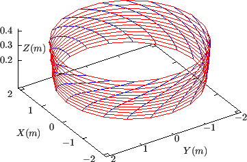
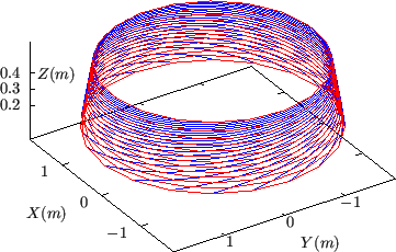
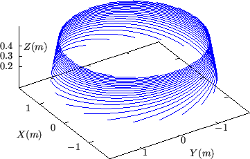
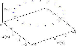
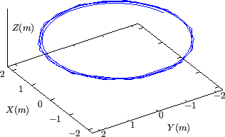
Figure 17 plots
![]() lines on the
lines on the
![]() isosurfaces,
which are chosen to be on the low-field-side midplane. On
isosurfaces,
which are chosen to be on the low-field-side midplane. On
![]() surface,
surface,
![]() lines are idential to
lines are idential to
![]() lines. On
lines. On
![]() surface,
surface,
![]() lines have large
lines have large ![]() shift. In my code,
shift. In my code,
![]() surface is chosen as the cut of
surface is chosen as the cut of ![]() and thus an inner
boundary connection condition for the perturbations is needed on this surface.
This connection condition is discussed in Sec. 8.2.1.
and thus an inner
boundary connection condition for the perturbations is needed on this surface.
This connection condition is discussed in Sec. 8.2.1.
 |