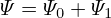
Consider the case that the boundary flux surface is circular with radius r = a and the center of the cirle at (R = R0,Z = 0). Consider the case 𝜀 = r∕R0 → 0. Expanding Ψ in the small parameter 𝜀,
|
| (591) |
where Ψ0 ∼ O(𝜀0), Ψ1 ∼ O(𝜀1). Substituting Eq. (591) into Eq. (590), we obtain
  r r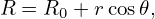 + + 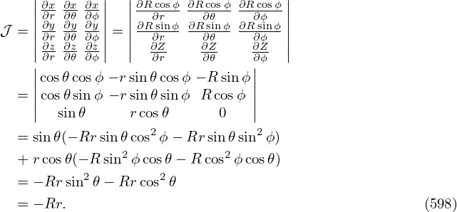 r r + +  + +  − −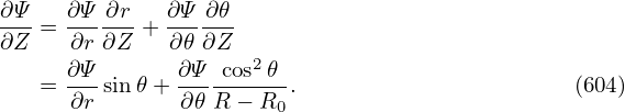 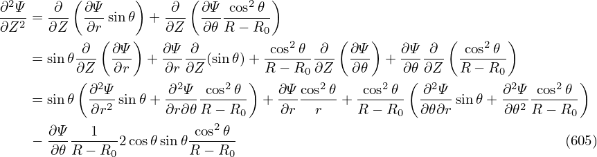 − −  = −μ0(R0+r cos𝜃)2P′(Ψ
0+Ψ1)−g′(Ψ0+Ψ1)g(Ψ0+Ψ1) = −μ0(R0+r cos𝜃)2P′(Ψ
0+Ψ1)−g′(Ψ0+Ψ1)g(Ψ0+Ψ1)
|
Multiplying the above equation by R02, we obtain
 | (592) |
Further assume the following orderings (why?)
 | (593) |
and
 | (594) |
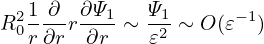
Using these orderings, the order of the terms in Eq. (592) can be estimated as
 | (595) |
 | (596) |
 | (597) |
 | (598) |
 | (599) |
 | (600) |
 | (601) |
 | (602) |
 | (603) |
The leading order (𝜀−2 order) balance is given by the following equation:
 | (604) |
It is reasonable to assume that Ψ0 is independent of 𝜃 since Ψ0 corresponds to the limit a∕R → 0. (The limit a∕R → 0 can have two cases, one is r → 0, another is R →∞. In the former case, Ψ must be independent of 𝜃 since Ψ should be single-valued. The latter case corresponds to a cylinder, for which it is reasonable (really?) to assume that Ψ0 is independent of 𝜃.) Then Eq. (604) is written
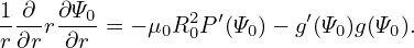 | (605) |
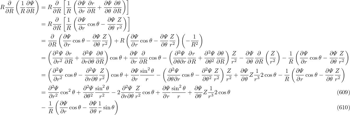
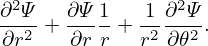
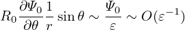
(My remarks: The leading order equation (605) does not corresponds strictly to a cylinder equilibrium because the magnetic field B = ∇Ψ0 ×∇ϕ + g∇ϕ depends on 𝜃.) The next order (𝜀−1 order) equation is
R02  r r +R02 +R02  −R0 −R0 cos𝜃 = −μ0R022R
0r cos𝜃P′(Ψ0)−μ0R04P′′(Ψ
0)Ψ1−R02[g′(Ψ
0)g(Ψ0)]′Ψ1 cos𝜃 = −μ0R022R
0r cos𝜃P′(Ψ0)−μ0R04P′′(Ψ
0)Ψ1−R02[g′(Ψ
0)g(Ψ0)]′Ψ1
|
![2
R21 ∂-r∂Ψ1+R2 1-∂-Ψ1+{μ0R4 P′′(Ψ0)+R2[g′(Ψ0)g(Ψ0)]′}Ψ1 = − μ0R22R0rcos𝜃P ′(Ψ0)+R0 ∂Ψ0cos𝜃
0r ∂r ∂r 0 r2 ∂𝜃2 0 0 0 ∂r](tokamak_equilibrium793x.png) | (606) |
 | (607) |
It is obvious that the simple poloidal dependence of cos𝜃 will satisfy the above equation. Therefore, we consider Ψ1 of the form
 | (608) |
where Δ(r) is a new function to be determined. Substitute this into the Eq. (), we obtain an equation for Δ(r),
 | (609) |
 | (610) |
 | (611) |
![( ) [ ( 2 ) ] 2
R201 d- rdΨ0dΔ- + ΔR20 1 d- rd-Ψ0 − 1-dΨ0(r) +R20d-Ψ0dΔ-+ d-{μ0R40P′(Ψ0)+R20g′(Ψ0)g(Ψ0)}Δ = − μ0R202R0rP′(Ψ0)+R0 dΨ0
r dr dr dr r dr dr2 r2 dr dr2 dr dr dr](tokamak_equilibrium799x.png) | (612) |
Using the identity
 ![[ ( )]
1 d- r dΨ0-
r dr dr](tokamak_equilibrium801x.png) = =   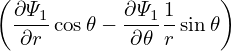 − − 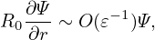 , ,
|
equation () is written as
![( ) [ ( ) ] 2
R201 d- rdΨ0dΔ- + ΔR20 d 1-d rdΨ0- +R20d-Ψ20dΔ-+ d-{μ0R40P ′(Ψ0)+R20g′(Ψ0)g(Ψ0)}Δ = − μ0R202R0rP′(Ψ0)+R0 dΨ0
r dr dr dr dr rdr dr dr dr dr dr](tokamak_equilibrium807x.png) | (613) |
Using the leading order equation (), we know that the second and fourth term on the l.h.s of the above equation cancel each other, giving
 | (614) |
 | (615) |
Using the identity
![[ ]
1 dr d ( dΨ0)2 dΔ 1d ( dΨ0dΔ ) d2Ψ0 dΔ
rdΨ-dr r dr-- dr- = rdr r-dr-dr + -dr2 dr ,
0](tokamak_equilibrium810x.png) | (616) |
equation (615) is written
![[ ( )2 ]
1-dr-d- r dΨ0- dΔ- = − μ02R0rP ′(Ψ0)+ -1-dΨ0,
rdΨ0 dr dr dr R0 dr](tokamak_equilibrium811x.png) | (617) |
![[ ]
1 d ( dΨ0)2 dΔ dP 1 ( dΨ0)2
⇒ rdr r dr-- dr- = − μ02R0rdr-+ R0- dr-- ,](tokamak_equilibrium812x.png) | (618) |
Using
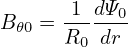 | (619) |
equation (618) is written
![1 d [ dΔ ] 1 dP B2
- -- rB2𝜃0--- = − μ02--r---+ --𝜃0.
r dr dr R0 dr R0](tokamak_equilibrium814x.png) | (620) |
![d [ dΔ] r ( dP (Ψ ) )
⇒ -- rB2𝜃0--- = --- − 2μ0r----0- + B2𝜃0 ,
dr dr R0 dr](tokamak_equilibrium815x.png) | (621) |
which agrees with equation (3.6.7) in Wessson’s book[27].