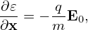
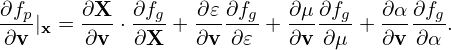
Since the definition of the guiding-center variables (X,𝜀,μ,α) involves the macroscopic (equilibrium) fields B0 and E0, to further simplify Eq. (33), we need to separate electromagnetic field into equilibrium and perturbation parts. Writing the electromagnetic field as
|
| (34) |
and
 | (35) |
then substituting these expressions into equation (33) and moving all terms involving the perturbed fields to the right-hand side, we obtain
where δR is defined by Next, let us simplify the left-hand side of Eq. (36). Note that
 | (38) |
where vE0 is defined by vE0 = cE0 × e∥∕B0, which is the E0 × B0 drift. Further note that
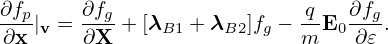
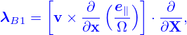
which can be combined with v ⋅ ∂fg∕∂X term, yielding v∥e∥⋅ ∂fg∕∂X. Finally note that Using Eqs. (38), (39), and (40), the left-hand side of equation (36) is written as which corresponds to Eq. (7) in Frieman-Chen’s paper[3]. [In Frieman-Chen’s equation (7), there is a term
 (E − E0) ⋅ v (E − E0) ⋅ v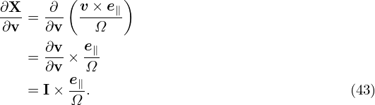
|
where E is the macroscopic electric field and is in general different from the E0 introduced when defining the guiding-center transformation. In my derivation E0 is chosen to be equal to the macroscopic electric field thus the above term does not appear.]
In expression (41), Lg is often called the unperturbed Vlasov propagator in guiding-center coordinates (X,𝜀,μ,α).
Using the above results, Eq. (36) is written as
 | (42) |
i.e.
It is instructive to consider some special cases of the above complicated equation. Consider the case that the equilibrium magnetic field B0 is uniform and time-independent, E0 = 0, and the electrostatic limit δB = 0, then equation (43) is simplified as
 | (46) |
![[ ]
∂fg + v⋅ ∂fg + v⋅ [λB1 + λB2]fg − q-E0∂fg
∂t ∂X m ∂𝜀( )
+ q-(E + v × B )× ( e∥)⋅ ∂fg+ -q(v × B )⋅ eα∂fg
m 0 0 Ω ∂X m 0 v⊥ ∂α
q ( ∂fg v⊥ ∂fg eα∂fg )
+ m-E0 ⋅ v-∂𝜀 + B--∂-μ + v--∂α
0 ⊥
= δRfg, (36)](nonlinear_gyrokinetic_equation40x.png)

![q v × B (e∥) ∂f ∂f
-------0 × -- ⋅--g = [(v× e∥)× e∥]⋅--g
m c Ω ∂X ∂f ∂X
= [v∥e∥ − v]⋅-g , (39)
∂X](nonlinear_gyrokinetic_equation43x.png)
![∂fg ∂fg ∂fg
∂t + ((v∥e∥ + VE0)⋅ ∂X +) v ⋅[λB1 + λB2]fg − Ω ∂α
-q v-⊥∂fg eα-∂fg
+ m E0 ⋅ B0 ∂μ + v⊥ ∂α ≡ Lgfg (41)](nonlinear_gyrokinetic_equation45x.png)
![∂fg + (v∥e∥ + VE0)⋅ ∂fg
∂t [ ( ) ∂X ]
+v ⋅ v × -∂- e∥ ⋅ ∂fg + ∂μ∂fg + ∂α-∂fg − Ω ∂fg
∂x Ω ∂X ∂x ∂μ ∂x ∂α ∂α
q ( v⊥ ∂fg eα∂fg)
+ m-E0 ⋅ B0-∂μ- + v⊥-∂α
( e ) ( )
= − q-(δE + v × δB)× -∥ ⋅ ∂fg− -q(v× δB )⋅ eα∂fg
m ( Ω ∂X ) m v⊥ ∂α
− q-δE ⋅ v∂fg + v⊥-∂fg + eα∂fg . (43)
m ∂𝜀 B0 ∂μ v⊥ ∂α](nonlinear_gyrokinetic_equation49x.png)