![q [ e∥] ∂Fg0 q ∂δL∂Fg0
LgδG = − m- (− ∇X ⊥ δL− v⊥ ⋅∇X ⊥δA )× Ω ⋅∂X--− m-∂t--∂-𝜀 + δRδFg,](nonlinear_gyrokinetic_equation100x.png)
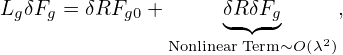
Plugging expression (94) into Eq. (82), we obtain
|
| (95) |
where Lg is given by Eq. (73), i.e.,
![Lg = -∂ + (v∥e∥ + VE0 )⋅-∂ + v⋅[λB1 + λB2 ]− Ω-∂
∂t ( ∂X ) ∂ α
+ -qE0 ⋅ v-⊥-∂-+ eα--∂- , (96)
m B0 ∂μ v⊥ ∂α](nonlinear_gyrokinetic_equation101x.png)
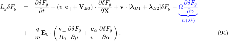
Expand δG as
| δG = δG0 + δG1 + …, |
where δGi ∼ O(λi+1)Fg0, and note that the right-hand side of Eq. (95) is of O(λ2), then, the balance on order O(λ1) requires
 | (97) |
i.e., δG0 is gyro-phase independent.
The balance on order O(λ2) requires (for the special case of E0 = 0):
Define the gyro-average operator ⟨…⟩α by
 | (99) |
where h = h(X,α,𝜀,μ) is an arbitrary function of guiding-center variables. The gyro-averaging is an integration in the velocity space. [For a field quantity, which is independent of the velocity in particle coordinates, i.e., h = h(x), it is ready to see that the above averaging is a spatial averaging over a gyro-ring.]
Gyro-averaging Eq. (98), we obtain
where use has been made of ⟨(v⊥⋅∇X)δA⟩α ≈ 0, where the error is of order higher than O(λ2). Note that v∥ = ± . Since B0 is approximately independent of α, so
does v∥. Using this, the first gyro-averaging on the left-hand side of the above equation is
written
. Since B0 is approximately independent of α, so
does v∥. Using this, the first gyro-averaging on the left-hand side of the above equation is
written
 | (101) |
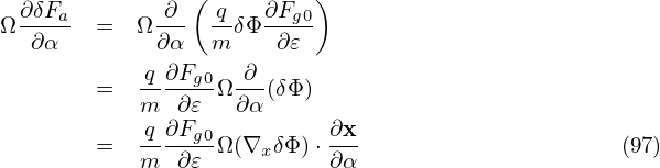
The second gyro-averaging on the left-hand side of Eq. (100) can be written as
![⟨v ⋅[λB1 + λB2]δG0⟩α = VD ⋅∇X δG0,](nonlinear_gyrokinetic_equation108x.png) | (102) |
where VD is the magnetic curvature and gradient drift (Eq. (102) is derived in Appendix xx, to do later). Then Eq. (100) is written
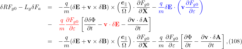
Next, we try to simplify the nonlinear term ⟨δRδFg⟩α appearing in Eq. (103), which is written as
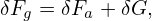
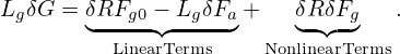 | (106) |
Accurate to O(λ2),the first term on the right-hand side of the above is zero. [Proof:
 | (108) |
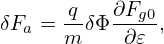
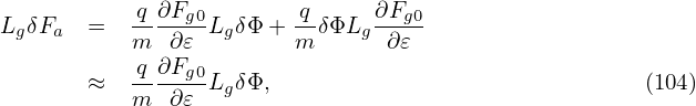
Using the expression of δR given by Eq. (37), the above expression is written as
where use has been made of ∂δG0∕∂α = 0. Using Eq. (92), we obtain
 | (110) |
The other two terms in Eq. (109) can be proved to be zero. [Proof:


![-q[ e∥]
⟨δRδG0 ⟩α = m ∇X ⊥⟨δL⟩α × Ω ⋅∇X δG0.](nonlinear_gyrokinetic_equation119x.png) | (113) |
Using this in Eq. (108), we obtain
![[ ]
⟨δRδFg⟩α = q- ∇X ⊥⟨δL⟩α × e∥ ⋅∇X δG0,
m Ω](nonlinear_gyrokinetic_equation120x.png) | (114) |
which is of O(λ2).
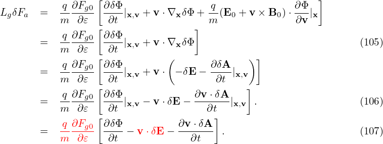
Using the above results, the gyro-averaged kinetic equation for δG0 is finally written as
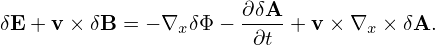
where VD is the equilibrium guiding-center drift velocity, ⟨…⟩α is the gyro-phase averaging operator, δL = δΦ− v ⋅δA, and δG0 = δG0(X,𝜀,μ,t) is gyro-angle independent and is related to the perturbed distribution function δFg by
 | (116) |
where the first term is called “adiabatic term”, which depends on the gyro-phase α via δΦ. Equation (115) is the special case (∂Fg0∕∂μ|𝜀 = 0) of the Frieman-Chen nonlinear gyrokinetic equation given in Ref. [3]. Note that the nonlinear terms only appear on the left-hand side of Eq. (115) and all the terms on the right-hand side are linear. The term
 | (117) |
consists of the perturbed E × B drift and magnetic fluttering term (refer to Sec. E.3).
![∂δG0-+ v∥e∥ ⋅ ∂δG0-+ v ⋅[λB1 + λB2]δG0
∂t [ ∂X ]
= −-q (− ∇X ⊥δL − v⊥ ⋅∇X δA )× e∥ ⋅ ∂Fg0 − q-∂δL-∂Fg0+ δR δFg. (98)
m Ω ∂X m ∂t ∂𝜀](nonlinear_gyrokinetic_equation103x.png)
![∂δG0 ⟨ ∂ δG0 ⟩
-∂t--+ v∥e∥ ⋅-∂X- + ⟨v⋅[λB1 + λB2 ]δG0⟩α
[ e ]
= −-q − ∇X ⊥⟨δL⟩α ×-∥ ⋅ ∂Fg0 − q-∂⟨δL⟩α∂Fg0 + ⟨δRδFg⟩α, (100)
m Ω ∂X m ∂t ∂𝜀](nonlinear_gyrokinetic_equation105x.png)
![[ ∂ ]
∂t + (v∥e∥ + VD )⋅∇X δG0
[ ]
= −-q − ∇X ⊥⟨δL⟩α × e∥ ⋅ ∂Fg0 − q-∂⟨δL⟩α ∂Fg0+ ⟨δRδFg⟩α. (103)
m Ω ∂X m ∂t ∂𝜀](nonlinear_gyrokinetic_equation109x.png)