Using Fg ≈ Fg0, equation (49) is written as
|
| (71) |
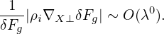
where δRδFg is a nonlinear term which is of order O(λ2) or higher, LgδFg and δRFg0 are linear terms which are of order O(λ1) or higher. The linear term δRFg0 is given by
 | (72) |
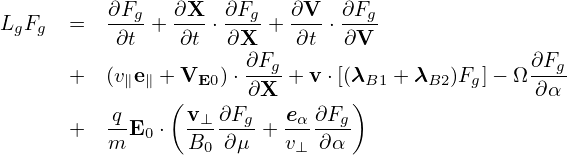
In obtaining (72), use has been made of ∂Fg0∕∂α = 0. Another linear term LgδFg is written as
where Ω∂δFg∕∂α is of order O(λ1) and all the other terms are of order O(λ2).Next, to reduce the complexity of algebra, we consider the easier case in which ∂Fg0∕∂μ = 0.
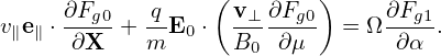
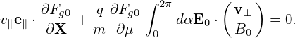
The balance between the leading terms (terms of O(λ)) in Eq. (71) requires that
 | (74) |
where δFa is a unknown distribution function to be solved from the above equation. It is ready to verify that
 | (75) |
is a solution to the above equation, accurate to O(λ). [Proof: Substitute expression (75) into the left-hand side of Eq. (74), we obtain
Using![∂x ∂ [ e∥(X )]
∂α-= ∂α-− v × Ω(X-)-
= ∂-[− v]× e∥(X-)
∂α Ω(X )
= − v⊥- (77)
Ω](nonlinear_gyrokinetic_equation85x.png)
As is discussed above, the terms of O(λ) can be eliminated by splitting a so-called adiabatic term form δFg. Specifically, write δFg as
 | (80) |
where δFa is given by (75), i.e.,
 | (81) |
which depends on the gyro-angle via δΦ and this term is often called adiabatic term. Plugging expression (80) into equation (71), we obtain
 | (82) |
Next, let us simplify the linear term on the right-hand side, i.e, δRFg0 −LgfδFa, (which should be of O(λ2) or higher because Ω∂δFa∕∂α cancels all the O(λ1) terms in δRFg0).
LgδFa is written
where the error is of order O(λ3). In obtaining the above expression, use has been made of e∥⋅∂Fg0∕∂X = 0, ∂Fg0∕∂X = O(λ1)Fg0, ∂Fg0∕∂α = 0, ∂Fg0∕∂μ = 0, and the definition of λB1 and λB2 given in expressions (20) and (21). The expression (83) involves δΦ operated by the Vlasov propagator Lg. Since δΦ takes the most simple form when expressed in particle coordinates (if in guiding-center coordinates, δΦ(x) = δΦ(X−v ×e∥∕Ω), which depends on velocity coordinates and thus more complicated), it is convenient to use the Vlasov propagator Lg expressed in particle coordinates. Transforming Lg back to the particle coordinates, expression (83) is written![q ∂F [ ∂δΦ q ∂Φ ]
LgδFa = ----g0 ---|x,v + v⋅∇x δΦ+ --(E0 + v× B0 )⋅---|x
m ∂𝜀 [ ∂t ] m ∂v
= q-∂Fg0 ∂δΦ|x,v + v⋅∇x δΦ (84)
m ∂𝜀 [ ∂t ( )]
q-∂Fg0 ∂δΦ- ∂δA-
= m ∂𝜀 ∂t |x,v + v⋅ − δE − ∂t |x,v
q ∂F [ ∂δΦ ∂v ⋅δA ]
= ----g0 ---|x,v − v⋅δE − ------|x,v . (85)
m ∂𝜀 [ ∂t ∂t]
= q-∂Fg0 ∂δΦ-− v⋅δE − ∂v-⋅δA- . (86)
m ∂𝜀 ∂t ∂t](nonlinear_gyrokinetic_equation91x.png)
The consequence of this is that, as we will see in Sec. 3.6, δG is independent of the gyro-angle, accurate to order O(λ1). Therefore, separating δF into adiabatic and non-adiabatic parts also corresponds to separating δF into gyro-angle dependent and gyro-angle independent parts.
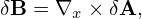
Let us rewrite the linear term (87) in terms of δΦ and δA. The δE + v ×δB term in expression (87) is written as
 | (88) |
Note that this term needs to be accurate to only O(λ). Then
 | (89) |
where the error is of O(λ2). Using the vector identity v ×∇x ×δA = (∇δA) ⋅v − (v ⋅∇)δA and noting v is constant for ∇x operator, the above equation is written
 | (90) |
Note that Eq. (22) indicates that ∇xδΦ ≈∇XδΦ, where the error is of O(λ2), then the above equation is written
 | (91) |
Further note that the parallel gradients in the above equation are of O(λ2) and thus can be dropped. Then expression (91) is written
where δL is defined by
 | (93) |
Using expression (92), equation (87) is written
![[ ]
δRF0 − LgδFa = − q- (− ∇X ⊥δL − v⊥ ⋅∇X ⊥δA) × e∥ ⋅ ∂Fg0 −-q∂δL-∂Fg0,
m Ω ∂X m ∂t ∂𝜀](nonlinear_gyrokinetic_equation99x.png) | (94) |
where all terms are of O(λ2).
![∂ δF ∂δF ∂ δF
Lg δFg =----g+ (v∥e∥ + VE0 )⋅--g-+ v⋅[λB1 + λB2 ]δFg − Ω---g
∂t ∂X ◟-∂◝α◜-◞
( ) O(λ1)
-q v⊥-∂δFg- -eα∂δFg-
+ m E0 ⋅ B0 ∂ μ + v⊥ ∂α , (73)](nonlinear_gyrokinetic_equation81x.png)
![( ) ( )
δRFg0 − LgδFa = − q(δE + v ×δB )× e∥ ⋅ ∂Fg0 − q-δE ⋅ v∂Fg0
m [ Ω ∂X ] m ∂ 𝜀
− q-∂Fg0 ∂δΦ-− v⋅δE − ∂v-⋅δA-
m ∂𝜀 ∂t ∂t
q (e∥) ∂Fg0 q ∂Fg0 [∂Φ ∂v ⋅δA ]
= − m(δE + v ×δB )× -Ω ⋅-∂X- − m--∂𝜀- ∂t-− --∂t--- , (87)](nonlinear_gyrokinetic_equation92x.png)