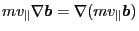
The phase-space Lagrangian for guiding-center motion was first given in
Littlejohn's paper[1], which takes the following form
 |
(1) |
where
 is the location of the guiding-center,
 is
the parallel (to magnetic field) velocity of the particle (will be proved
later that
is also the parallel velocity of the guiding
center)
is
the parallel (to magnetic field) velocity of the particle (will be proved
later that
is also the parallel velocity of the guiding
center)
 with
with  the perpendicular (to
magnetic field) velocity of the particle,
the perpendicular (to
magnetic field) velocity of the particle,  is the gyrophase,
 with
with  being the charge number and
  being the elementary
charge,
being the elementary
charge,
 . Note that here the (phase-space)
Lagrangian of guiding center is considered to be a function of variables
. Note that here the (phase-space)
Lagrangian of guiding center is considered to be a function of variables
 , and
, and  . Also note that three
variables, ,
. Also note that three
variables, ,
 and
and  happens not to appear
in Eq. (1). Further note that the explicit dependence of
happens not to appear
in Eq. (1). Further note that the explicit dependence of
 on
and is through the electromagnetic field
on
and is through the electromagnetic field
 ,
,  , and the frequency
  . The Euler-Lagrange
equation corresponding to variable
. The Euler-Lagrange
equation corresponding to variable  is written as
 |
(2) |
which, after evaluating the partial derivatives, is reduced to
 |
(3) |
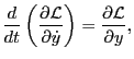
which indicates as expected that the time change rate of the gyrophase
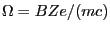
equals the cylcotron frequency . The Euler-Lagrange equation
corresponding to the variable is written as
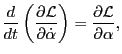 |
(4) |
which can be written as
 |
(5) |
which indicats that the magnetic moment
 is a constant of
the motion. The Euler-Lagrange equation for the variable
is
is a constant of
the motion. The Euler-Lagrange equation for the variable
is
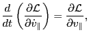 |
(6) |
which can be simplified to
 |
(7) |
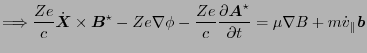
which indicates that
is also the parallel velocity of the
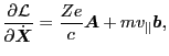
guiding center. Next, consider the Euler-Lagrange equation corresponding to
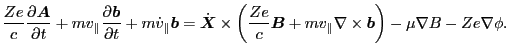
the coordinate
, which is given by
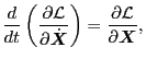 |
(8) |
which should be understood as a shorthand of the three Euler-Lagrange
equations coorresponding to three coordinates. Is the above equation still
valid in arbitrary coordinates system if we consider
 and
and
 as gradient
operators? The answer is yes. However it is not trivial for me to find the
proof (the proof is provided in Sec. (4)). Using Eq.
(1) and vector identies, we obtain
as gradient
operators? The answer is yes. However it is not trivial for me to find the
proof (the proof is provided in Sec. (4)). Using Eq.
(1) and vector identies, we obtain
 |
(9) |
and
 |
(10) |
where
 . Using Eqs.
(9) and (10), Eq. (8) is written as
. Using Eqs.
(9) and (10), Eq. (8) is written as
 |
(11) |
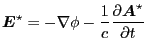
Using
 and
and
 , the second last
term can be reduced to
, the second last
term can be reduced to
 . Then Eq. (11) is written
as
. Then Eq. (11) is written
as
 |
(12) |
Noting that
 (this is because
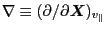 , i.e., holding
constant), so
that the second term on the right-hand side of the above equation is canceled
by terms on the right-hand, yielding
, i.e., holding
constant), so
that the second term on the right-hand side of the above equation is canceled
by terms on the right-hand, yielding
 |
(13) |
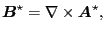
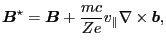
Equation (13) can be further written in compact form by defining
new magnetic-like and electric-like quantities. Define
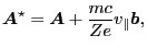 |
(14) |
and
 |
(15) |
then
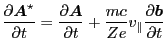 |
(16) |
 |
(17) |
(Note that the time partial differential does not operate on
because it is an independent variables.) Using these, Eq. (13) is
written as
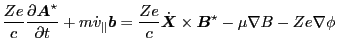 |
(18) |
 |
(19) |
Define
 |
(20) |
then Eq. (19) is written as
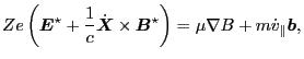 |
(21) |
which agrees with Eq. (23) of Porcelli's paper[1].
Subsections
YouJun Hu
2014-05-19